Computer Architecture 是一個 end-to-end 的優化,有非常多因素都會影響到他的效能,不管是往上的 OS, application,往下的電路
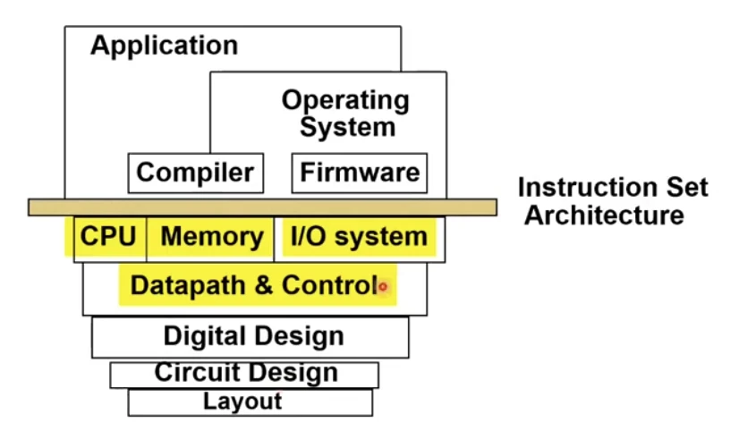 Computer Architecture in the whole computer
Application#
每當有新的 Application 出來都會需要新的 architecture 來做適應
- 1990’ 多媒體, 3D, video: MMS, SSE, GPU
- 2000’ RMS (Recognition, Mining, Sythesis): Multi-core, GPGPU, 3D memory
- 2010’ Machine learning, data analytics: Domain-specific architecture, e.g. DNN accelerators
現代的 architecture 必須要跟著現代應用走,並且需要做預測
Technology#
根據科技演進,整個
CostPerformance
的比值越來越高,舉例來說
- 1951 Vacuum tube: 1
- 1965 Transistor: 35
- 1975 Integrated circuit (IC): 900
- 1995 Very large scale IC (VLSI): 2400000
- 2013 Ultra large scale IC: 250000000000
根據 Moore’e Law,他做了一個 prediction,每年,同樣 IC 下的 transistor 數量會每年增加一倍,而現實則是大約每 18 個月會 double 一次
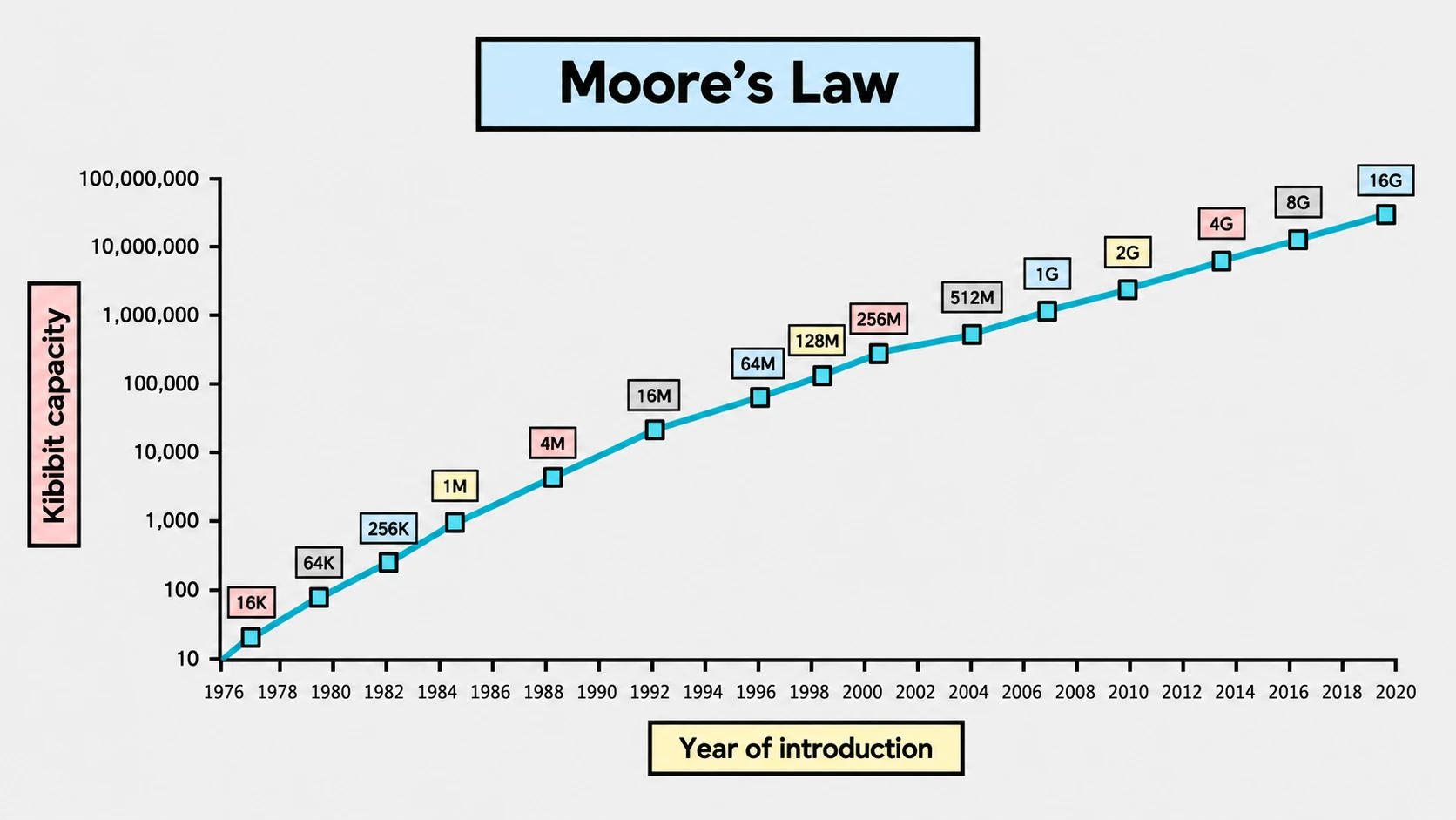 Moore'e Law
但摩爾定律已經快要失效了,可能需要靠 Parallel Computing 或是 Quantum Computing 的努力
Computer Engineering Methodology#
在設計一個系統的時候我們必須先知道我們想參照哪個 factor,並且這個 factor 需要可以 量化 (Quantify),因此我們需要進行 分析 (Analysis) 才能對 solution space 做縮減,因此系統設計其實分析佔一半,我們必須設計出一套良好的指標,也就是 Metric,並且我們必須要有一套 Benchmark 標準
Response Time and Throughput#
這兩個是 CPU 非常重要的 metric
- Response Time 是 computing platform 解決一個 task 需要的時間
- Throughput 是每單位時間內 computing platform 能解決的任務數量
兩者有相關,但他們並不完全相等,比如說
- 更新 processor 成下一代,可以增加 throughput 也可以減少 response time
- 增加 processor 的數量會增
- 家 throughput 但並不會增加 response time
我們首先 Define Performance 是
Performance=Execution time1
所以當我們說 ”X is n time faster than Y“,就代表
PerformanceYPerformanceX=Execution timeXExecution timeY=n
Execution time#
Execution time 分成兩種
- Elapsed time:所有運行的時間,包含 CPU processing, I/O, OS overhead, idle time
- CPU time:只有真正在執行的時間,把所有 I/O, idle 都消掉,而這個又可以細分成 System CPU time 跟 User CPU time
CPU time#
我們定義
CPU time=CPU Clock Cycles×Clock Cycle time=Clock RateCPU Clock Cycle
首先我們來看看 Clock
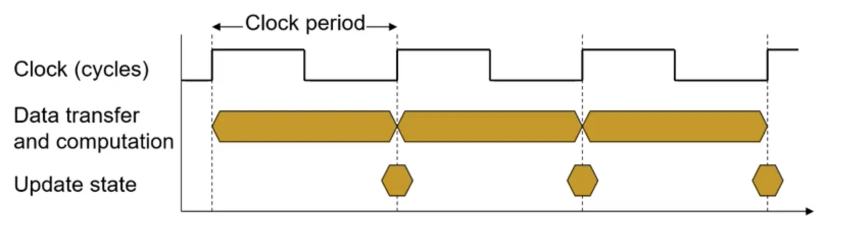 CPU clocking
一個 period 就是一個 clock cycle,一個 clock 結束的時候,也就是 rising edge,我們會 update digital module 的 state
- Clock period:Duration of a clock cycle
- Clock frequency:Cycles per second
從這個式子,有幾個因素可以增進 CPU time(變小)
- 減少 Clock cycles
- 增加 Clock rate
但硬體設計師通常需要在這兩個變數之間做 trade-off,後面會提到二者關聯
Instruction Count and CPI#
剛剛我們有一個定義
CPU time=CPU Clock Cycles×Clock Cycle time
現在我們繼續定義這些 terms,並且延伸定義 CPU time
Clock CyclesCPU Time=Instruction Count×Cycles per Instruction (CPI)=Instruction Count×CPI×Clock Cycle Time=Clock RateInstruction Count×CPI
一樣從這個式子,有幾個因素可以增進 CPU time
- 我們寫的 Algorithm 一定會影響到 Instruction count
- Compiler 的 Optimization 也會影響到 Instruction count
不同的 Instruction Set Architecture (ISA) run 不同的 instruction 需要ㄉㄜ cycle 數量是不一樣的,所以我們需要更精確的 CPI 定義,因為我們需要把不同的 Instruction 分類成 n 個 class
Clock Cycles=i=1∑n(CPIi×Instruction Counti)
而我們還可以定義平均的 CPI 讓我們更能夠衡量機器的好壞
CPI=Instruction CountClock Cycles=i=1∑nCPIi×Relative frequencyInstruction CountInstruction Counti
總的來看 CPU Performance 可以歸於一個公式
CPU time=ProgramSeconds=Program#Instructions×Instruction#Cycles×CycleSeconds
| Factor/Metric | Inst Count | CPI | Clock Rate |
|---|
| Algorithm | V | V | |
| Programming Language | V | V | |
| Compiler | V | V | |
| ISA (Instruction Set Architecture) | V | V | V |
軟體層面影響 CPI, Instruction count 很大,而 Clock rate 只會被 ISA 或是 hardware 影響
上面三個 Metric 少考慮任何一個,我們都無法判斷機器的 performance,必須要三者皆考慮到
Power#
在 CMOS IC 裡面 Power 的定義如下
Power≈Capacitive load×V2×f
這裡的 V 是 Votage, f 是 frequency,這裡的 Power 是 dynamic power,隨著科技進步我們讓 5V 下降到 1V 但 frequency 上升了 1000 倍
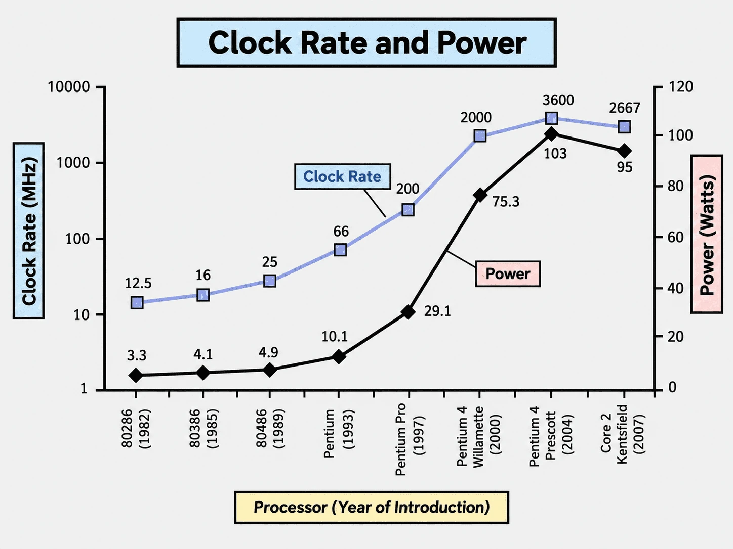 Power Trend
因為我們沒辦法再繼續 reduce power 了也沒辦法再 remove more heat 我們遇到了一個 power wall 也就是無法繼續提升 frequency
Single processor 的架構在後期無法用 pipeline 再提升他的性能,因為遇到了 power wall,為了要考慮到 overall 的 performance 以及 power 這個 factor 人類開始嘗試 many core 的架構
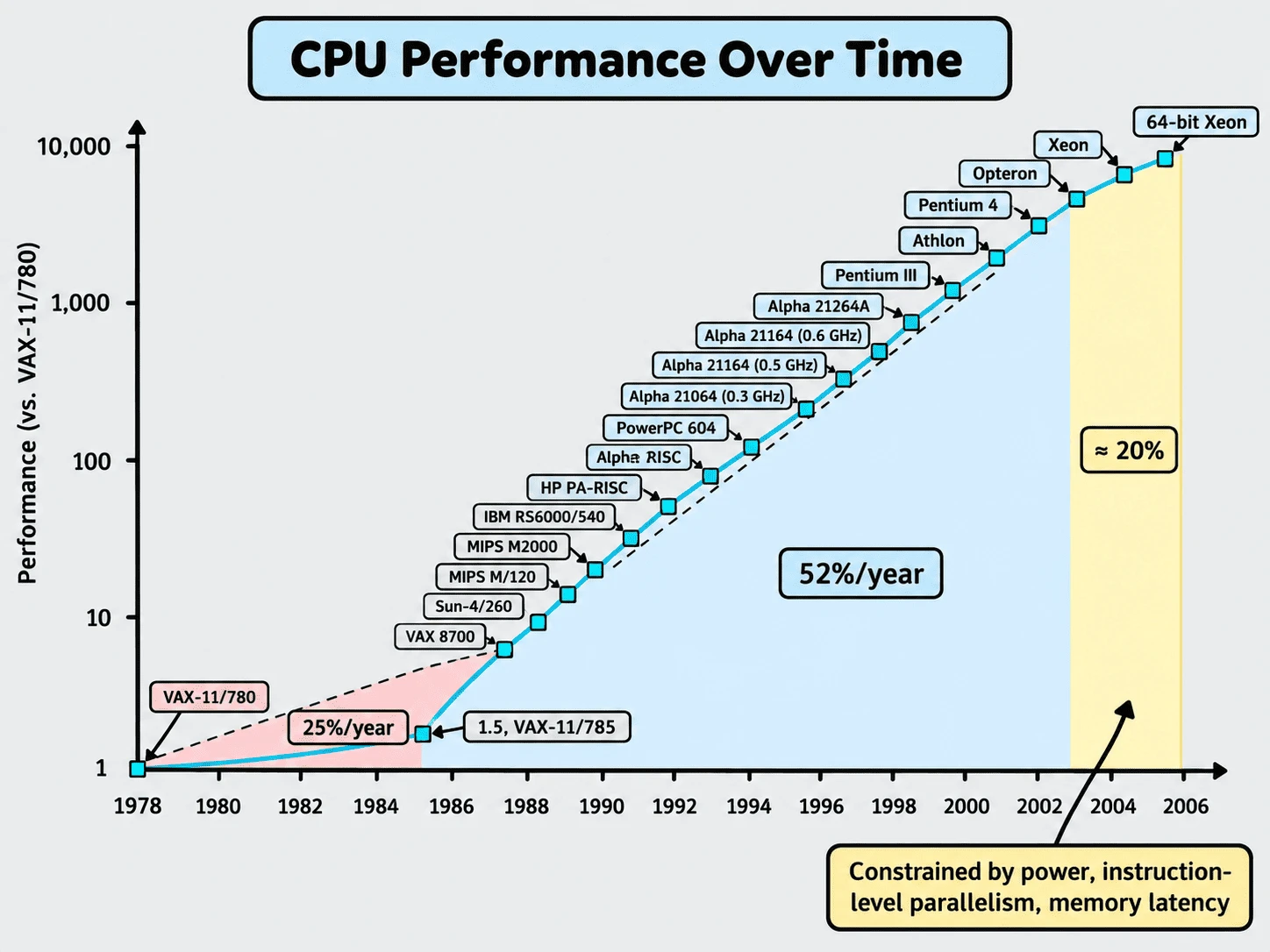 Uniprocessor performance
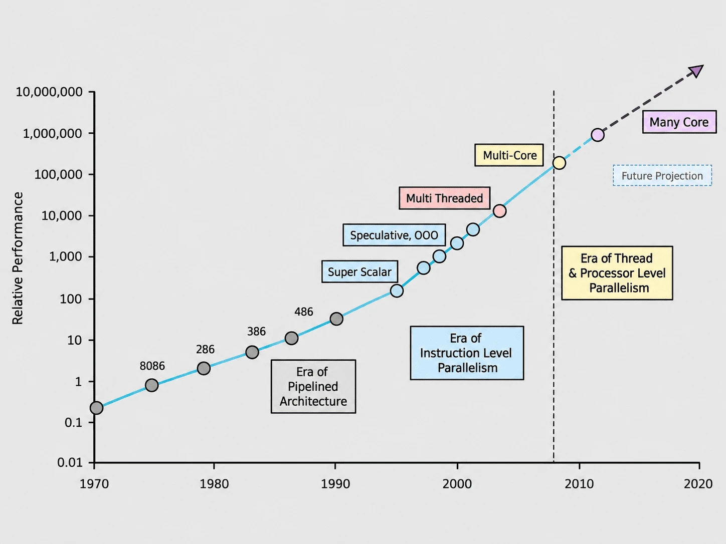 CPU performance on different Era
Multi-core for Power#
為什麼 Multi-core 會比較好呢,為了做推導,我們先複習兩個觀念,Power 跟 Energy
PowerEnergy=dtdEnergy(Watt=Joule/second)=Power×Time(Joule)
Power 描述的是能量消耗的速率,也就是某一時刻系統消耗能量有多快;而 Energy 則表示完成整個 task 過程中所消耗的總能量。
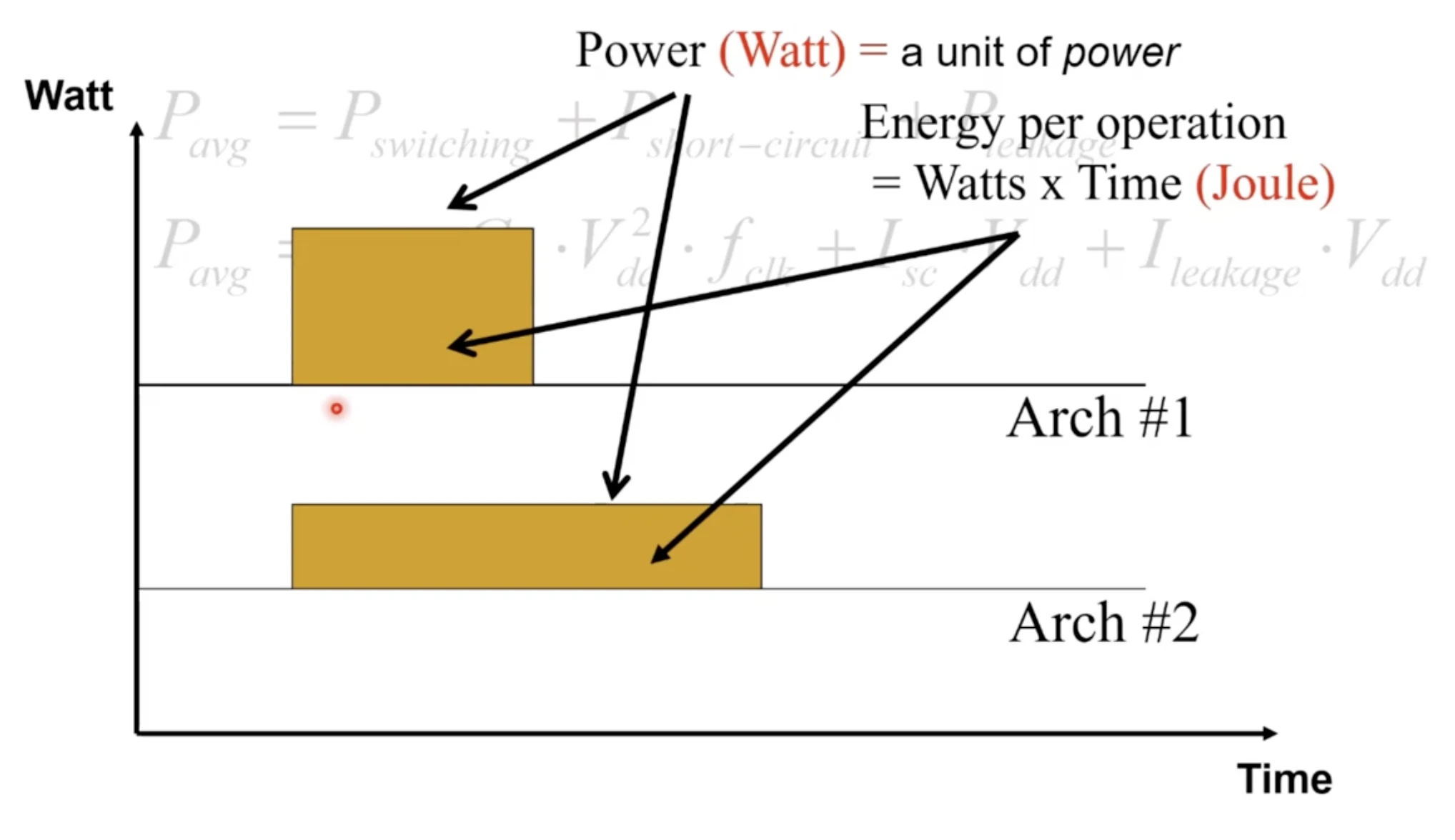 Power and Energy
因此,我們在討論 Energy Efficiency 時,關心的是:在完成相同工作量的情況下,能不能消耗更少的 Energy,或者換個角度來說,在相同的 Energy budget 下,能不能完成更多的工作。
因為 Voltage 跟 Frequency 也有一定程度的正相關,所以我們還是用可以簡單把 Power 規約成 f3
我們希望維持相同的 performance / throughput。在理想情況下,如果工作可以完全平行化,兩個 core 各跑一半的 frequency,總計算能力仍可以和原本一個 core 相同,在這樣的情況下計算,我們可以發,parallel 的 computing 只需要 1/4 的 Energy
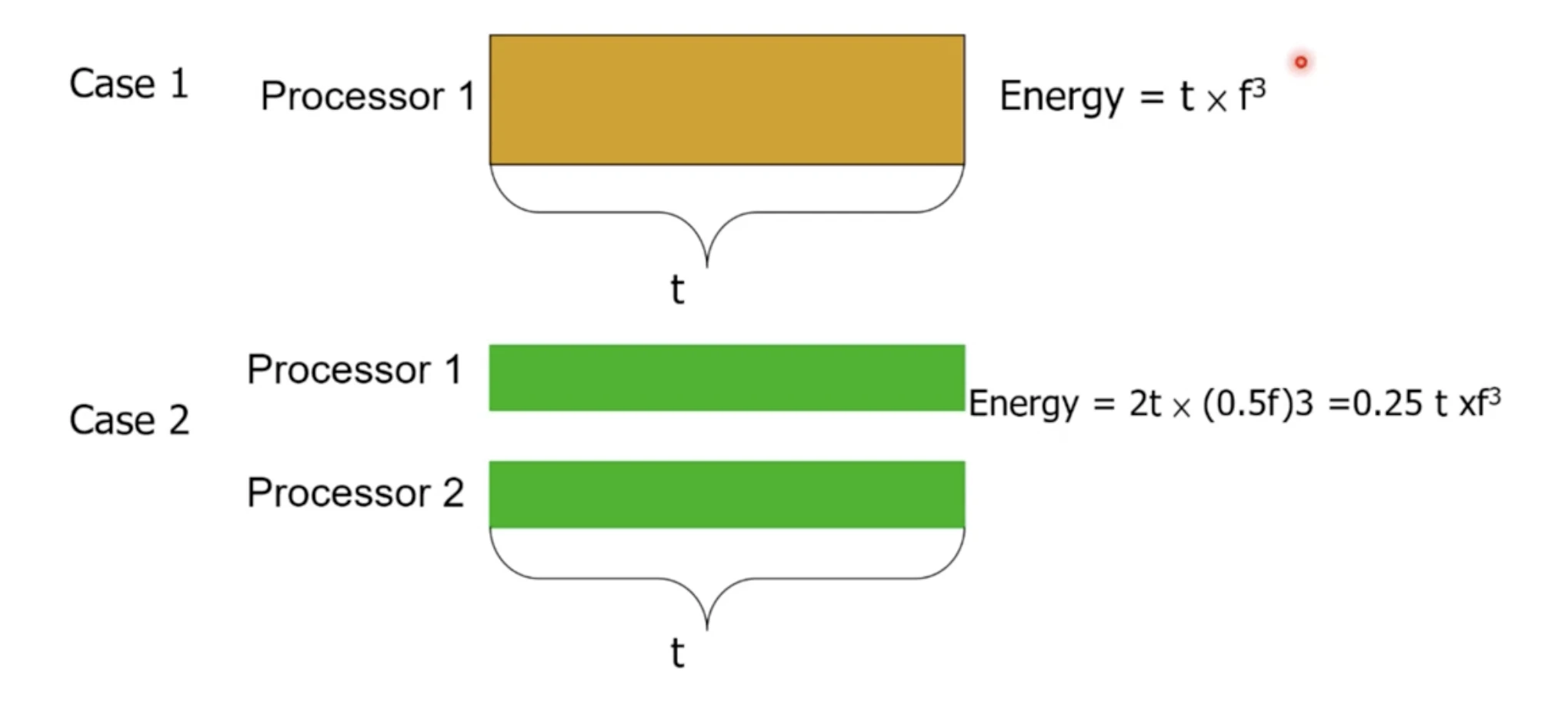 Power on Multi-core
雖然我們知道 Multi-core 很好,但這樣的 architecture 不像 Instruction level 的 parallelism,programmer 不需要 aware,可以像平常一樣。Multi-core 不一樣,他需要 programmer 做 parallel programming 還需要考慮很多細節
- Load balancing
- Optimize communication and synchronization
Cost#
Chip 是方形的可以最大化它可以填到晶圓的數量
- 還沒封裝的晶片叫做Die
- 一個Die上面可能有很多核心,有單一核心有瑕疵還是可以當成次級品賣
良率 Yeild 的基礎定義就是 working die (晶片) per wafer (晶圓) 的比率
以下是 IC 製程的細節
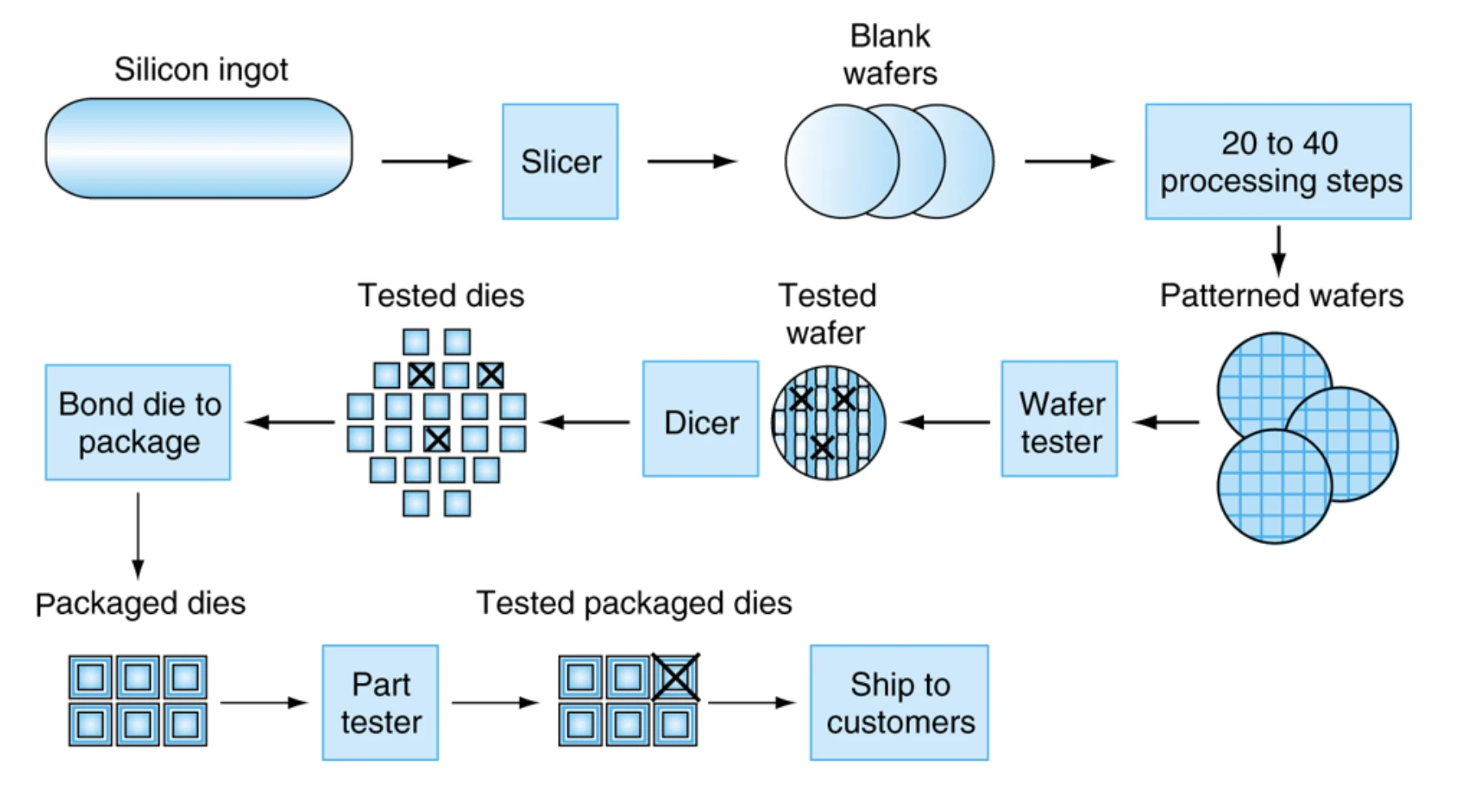 IC Manufacturing
以下是 cost 和 yeild 之間的關係
Cost per DieDie per WaferYield=Dies per Wafer×YieldCost per Wafer≈Die AreaWafer Area=(1+(Defects per Area×2Die Area))21
從上面這個公我們可以看出,Die area 要越小越好,並且 Cost 和 Yeild 之間是 nonlinear 的關係
- Wafer cost, area 都是固定的
- Defect rate 跟這個公式有很大關係,而這由 manufacturing process 有很大關係
Benchmark#
SPEC CPU Benchmark#
CPU 會跑的 application 很多,而 SPEC (Standard Performance Evaluation Corp) CPU Benchmark 是 SPEC 這個組織認為 CPU 應該會跑的一系列 application 的集合,他有以下幾個特點
- 是一個 general purpose 的 benchmark(不像某些 embedding system 的 benchmark)
- 因為想了解的是真實的 user 體驗,計算的是 elapsed time,但他有特化所短 I/O 時間 (compute-intensive),所以主要測量的還是 CPU performance
- 包含 integer application (CINT), floating-point application (CFP)
以下是詳細的 Benchmark 內容,可以看到有不少難度高的 task
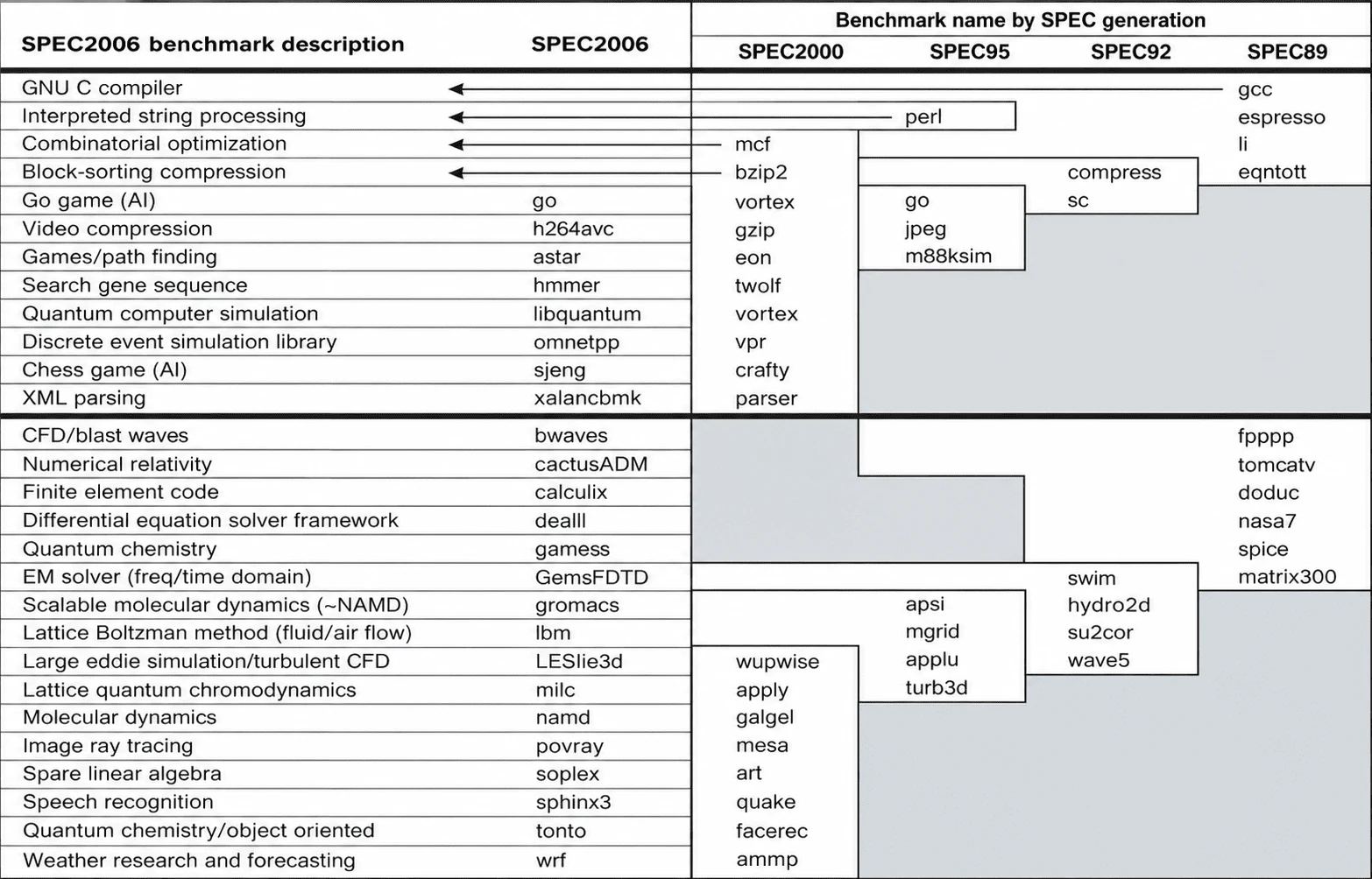 SPEC benchmark
Summarize 整個 benchmark 的方法有很多種,也許我們可以直接算 arithmetic average,但很明顯他會被用時最長的 task dominate,所以我們要先做 normalize
SPECRatio=TComputer being RatedTRefernce Computer
SPECRatio 越高越好,因為時間越低越好,Performance 越高越好,接下來我們需要決定 reference machine 要用哪台,看一下以下推導
SPECRatioBSPECRatioA=Execution timeBExecution timereferenceExecution timeAExecution timereference=Execution timeAExecution timeB=PerformanceBPerformanceA
我們其實不會因為不一樣的 Reference machine 而有不同的 ratio 比例,所以其實沒有差,算出每個 Task 的 SPECRatio 後,用幾何平均做加權
Geometry Mean=(i=1∏nSPECRatioi)
SPEC Power Benchmark#
是一個專門在測量 server power 的 benchmark,實際上跑的是 SPECJBB (Java Business Application) benchmark,這個 bench mark 可以調整 workload,讓 server 在不同的 load level 下運作,並同時測量
- ssj_ops:server 在單位時間內完成的 operation 數量
- Power:server 在該 load level 下消耗的功率
Overall ssj_ops per Watt=∑i=010Power i∑i=010ssj_opsi
我們最終算的是 Energy Efficiency,也就是 #operation per Watt
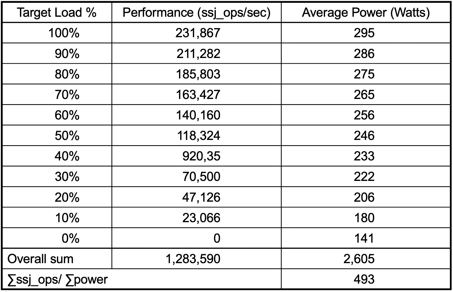 SPEC Power benchmark
值得注意的是即便 loading 是 0%,他也是滿載情況下的 1/2,這就是 ** **
Pitfall and Fallacy#
Amdahl’s Law#
Timproved=NTaffected+Tuneffected
這是一個出現過很多次的公式,parallel 的結果不會影響到不能平行化的部分
 To improve performance with parallelism
從這個公式可以看到,優化的一大重點,是選擇 optimize 的 target,一定要選擇值得優化的部分(common case)去做優化,而不要亂亂選,要先做 analysis
Low Power at Idle#
從剛剛的例子就可以看出,其實 Idle 的時候,Power 消耗還是非常大,通常情況下一個 server 的 loading 會在 10%~50% 之間,所以我們希望可以增加 energy efficiency 的區段會在這裡
MIPS 是 Millions of Instructions Per Second,但這並不能當作比較基準,因為每個 architecture 的 CPI 是不一樣的,相當於只考慮了兩個因素,第三個沒考慮到
MIPS=Execution time×106Instruction count=Clock rateInstruction count×CPI×106Instruction count=CPI×106Clock rate
Summary#
8 Design Principle for Computer Architecture#
- design for Moore’s Law
- use abstraction to simplify design
- make the common case fast
- performance via parallelism
- performance via pipelining
- performacne via prediction
- hierarchy of memories
- dependability via redundency